Tutorial

Quickstart

csaps provides object-oriented API for computing and evaluating univariate, multivariate and nd-gridded splines, but in most cases we recommend to use a shortcut function csaps() for smoothing data and computing splines.

Firstly, we import csaps() function and other modules for our examples and also define the function that will produce univariate data:

import numpy as np
import matplotlib.pyplot as plt
from mpl_toolkits.mplot3d import Axes3D

from csaps import csaps


def univariate_data(n=25, seed=1234):
    np.random.seed(seed)
    x = np.linspace(-5., 5., n)
    y = np.exp(-(x/2.5)**2) + (np.random.rand(n) - 0.2) * 0.3
    return x, y

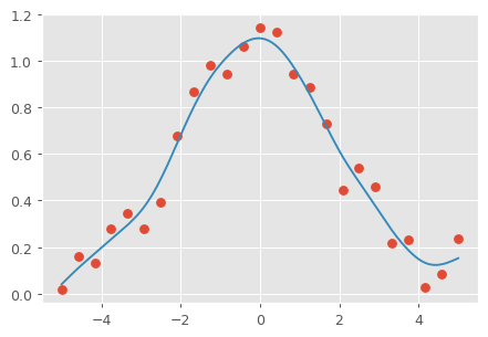
Univariate Smoothing

Univariate data are two vectors: X and Y with the same size. X is data sites, Y is data values. X-values must satisfy the condition: \(x1 < x2 < ... < xN\)

It is a simple example how to smooth univariate data:

x, y = univariate_data()
xi = np.linspace(x[0], x[-1], 150)

yi = csaps(x, y, xi, smooth=0.85)

plt.plot(x, y, 'o', xi, yi, '-')

Multivariate Smoothing

Also we can smooth multivariate (n-dimensional) data using the same function.

The algorithm supports computing and evaluating spline for multivariate data with vectorization. You can compute smoothing splines for X, Y data where X is data site vector and Y is ND-array of data value vectors.

The example of data:

# data sites
x = [1, 2, 3, 4]

# 3 data vectors (3-D)
y = [
    (2, 4, 6, 8),
    (1, 3, 5, 7),
    (5, 1, 3, 9),
]

By default, the shape of Y array must be: (d0, d1, ..., dN) where dN must equal to X vector size. Also you can use axis parameter to set the data values axis for Y array.

In this case the smoothing spline will be computed for all Y data vectors at a time. The same weights vector and the same smoothing parameter will be used for all Y data.

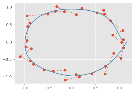
2-D data example:

np.random.seed(1234)
theta = np.linspace(0, 2*np.pi, 35)
x = np.cos(theta) + np.random.randn(35) * 0.1
y = np.sin(theta) + np.random.randn(35) * 0.1
data = [x, y]
theta_i = np.linspace(0, 2*np.pi, 200)

data_i = csaps(theta, data, theta_i, smooth=0.95)
xi = data_i[0, :]
yi = data_i[1, :]

plt.plot(x, y, ':o', xi, yi, '-')

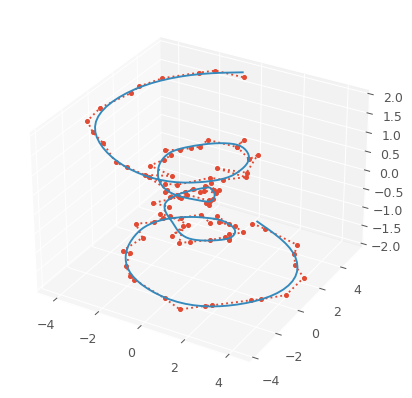
3-D data example:

np.random.seed(1234)
n = 100
theta = np.linspace(-4 * np.pi, 4 * np.pi, n)
z = np.linspace(-2, 2, n)
r = z ** 2 + 1
x = r * np.sin(theta) + np.random.randn(n) * 0.3
y = r * np.cos(theta) + np.random.randn(n) * 0.3
data = [x, y, z]
theta_i = np.linspace(-4 * np.pi, 4 * np.pi, 250)

data_i = csaps(theta, data, theta_i, smooth=0.95)
xi = data_i[0, :]
yi = data_i[1, :]
zi = data_i[2, :]

fig = plt.figure(figsize=(7, 4.5))
ax = fig.add_subplot(111, projection='3d')
ax.set_facecolor('none')
ax.plot(x, y, z, '.:')
ax.plot(xi, yi, zi, '-')

N-D grid Smoothing

Finally, using the same function we can smooth n-d gridded data.

The algorithm can make smoothing splines for n-d gridded data smoothing. In this case the algorithm makes coordinatewise smoothing (tensor-product of univariate splines coefficients).

X-data must be a sequence of vectors for each dimension. Y-data must be n-d array.

The example of data:

x = [
    (-2, -1, 0, 1, 2),    # X-grid data sites
    (-2, -1, 0, 1, 2),    # Y-grid data sites
    (-2, -1, 0, 1, 2),    # Z-grid data sites
]

y = np.random.rand(5, 5, 5)  # 5x5x5 3-D grid data values

Also you can set the smoothing parameter for each dimension:

smooth = [
    0.95,  # the smoothing parameter for X
    0.83,  # the smoothing parameter for Y
    0.51,  # the smoothing parameter for Z
]

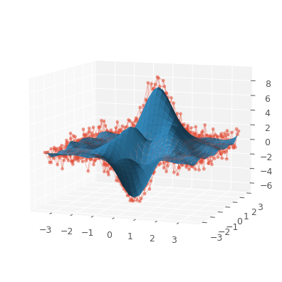
Surface data example:

np.random.seed(1234)
xdata = [np.linspace(-3, 3, 41), np.linspace(-3.5, 3.5, 31)]
i, j = np.meshgrid(*xdata, indexing='ij')
ydata = (3 * (1 - j)**2. * np.exp(-(j**2) - (i + 1)**2)
         - 10 * (j / 5 - j**3 - i**5) * np.exp(-j**2 - i**2)
         - 1 / 3 * np.exp(-(j + 1)**2 - i**2))
ydata = ydata + (np.random.randn(*ydata.shape) * 0.75)

ydata_s = csaps(xdata, ydata, xdata, smooth=0.988)

fig = plt.figure(figsize=(7, 4.5))
ax = fig.add_subplot(111, projection='3d')
ax.set_facecolor('none')
c = [s['color'] for s in plt.rcParams['axes.prop_cycle']]
ax.plot_wireframe(j, i, ydata, linewidths=0.5, color=c[0], alpha=0.5)
ax.scatter(j, i, ydata, s=10, c=c[0], alpha=0.5)
ax.plot_surface(j, i, ydata_s, color=c[1], linewidth=0, alpha=1.0)
ax.view_init(elev=9., azim=290)

Summary

In all the smoothing examples above we are used the following csaps() signature:

yi = csaps(x, y, xi, smooth)

where

• x – the data sites vector for univariate/multivariate data and a sequence of vectors for nd-gridded data. x-values must satisfy the condition: x1 < x2 < ... < xN

• y – the data values. For univariate case it is vector with the same size as x, for multivariate case it is a sequence of vectors or nd-array, and for nd-gridded data it is nd-array

• xi – the data sites for smoothed data (output mesh). It is shape-like x and in the same range as x, but usually it has more interpolated points

• smooth – the smoothing parameter in the range [0, 1]

Advanced Usage

Automatic Smoothing

If we want to smooth the data without specifying the smoothing parameter we can use the following signature:

yi, smooth = csaps(x, y, xi)

In this case the smoothing parameter will be computed automatically and will be returned in the function result. In this case the function will return AutoSmoothingResult named tuple: AutoSmoothingResult(values, smooth).

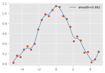
The example of auto smoothing univariate data:

x, y = univariate_data()
xi = np.linspace(x[0], x[-1], 51)

smoothing_result = csaps(x, y, xi)

yi = smoothing_result.values
smooth = smoothing_result.smooth

plt.plot(x, y, 'o')
plt.plot(xi, yi, '-', label=f'smooth={smooth:.3f}')
plt.legend()

In ND-gridded data case we can use auto smoothing for all dimensions or the particular dimensions:

smooth = [
    0.95,
    None,  # auto smoothing only for Y
    0.85,
]

...

smoothing_result = csaps(x, y, xi, smooth=smooth)

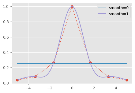
Bounds of Smoothing Parameter

The smoothing parameter \(p\) should be in range \([0, 1]\) where bounds are:

• 0: The smoothing spline is the least-squares straight line fit to the data

• 1: The cubic spline interpolant with natural boundary condition

The following example demonstartes these two boundary cases:

x = np.linspace(-5., 5., 7)
y = 1 / (1 + x**2)
xi = np.linspace(x[0], x[-1], 150)

yi_0 = csaps(x, y, xi, smooth=0)
yi_1 = csaps(x, y, xi, smooth=1)

plt.plot(x, y, 'o:')
plt.plot(xi, yi_0, '-', label='smooth=0')
plt.plot(xi, yi_1, '-', label='smooth=1')
plt.legend()

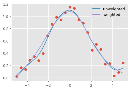
Weighted Smoothing

If we want to use error measure weights while computing spline, we can use the following signatures:

yi = csaps(x, y, xi, weights, smooth)
yi, smooth = csaps(x, y, xi, weights)
spline = csaps(x, y, weights)
spline = csaps(x, y, weights, smooth)

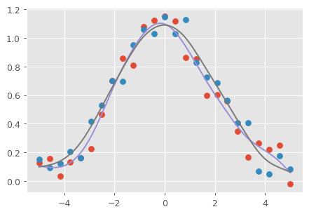
The example of weighted smoothing univariate data:

x, y = univariate_data()
xi = np.linspace(x[0], x[-1], 150)

w = np.ones_like(x) * 0.5
w[-7:] = 0.1
w[:7] = 0.1
w[[10,13]] = 1.0
w[[11,12]] = 0.1

yi = csaps(x, y, xi, smooth=0.85)
yi_w = csaps(x, y, xi, weights=w, smooth=0.85)

plt.plot(x, y, 'o')
plt.plot(xi, yi, '-', label='unweighted')
plt.plot(xi, yi_w, '-', label='weighted')
plt.legend()

In n-d gridded data case we can use the same weights for all dimensions or different weights for each dimension.

Axis Parameter

axis parameter specifies Y-data axis for computing spline in multivariate/vectorize data cases (axis along which Y-data is assumed to be varying). By default axis is equal to -1 (the last axis). In other words, y.shape[axis] must be equal to x.size.

For example, the following code will raise ValueError without axis parameter:

x, y1 = univariate_data(seed=1327)
x, y2 = univariate_data(seed=2451)

# We stack y-data as MxN array
y = np.stack((y1, y2), axis=1)

print('x.size:', x.size)
print('y.shape:', y.shape)

xi = np.linspace(x[0], x[-1], 150)

# yi = csaps(x, y, xi, smooth=0.8)  # --> ValueError: invalid "ydata" shape for given "xdata"
yi = csaps(x, y, xi, smooth=0.8, axis=0)

plt.plot(x, y, 'o', xi, yi, '-')

Note

axis parameter is ignored in ND-gridded data cases.

Smooth normalization

New in version 1.1.0.

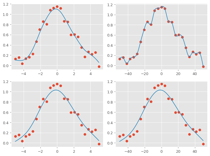
We can use normalizedsmooth option to normalize smooth parameter. If normalizedsmooth is True, the smooth parameter is normalized such that results are invariant to xdata range and less sensitive to nonuniformity of weights and xdata clumping.

Let’s show it on a simple example.

x1, y = univariate_data(seed=1327)
x2 = x1 * 10

xi1 = np.linspace(x1[0], x1[-1], 150)
xi2 = np.linspace(x2[0], x2[-1], 150)

yi1 = csaps(x1, y, xi1, smooth=0.8)
yi2 = csaps(x2, y, xi2, smooth=0.8)

yi1_n = csaps(x1, y, xi1, smooth=0.8, normalizedsmooth=True)
yi2_n = csaps(x2, y, xi2, smooth=0.8, normalizedsmooth=True)

f, ((ax1, ax2), (ax3, ax4)) = plt.subplots(2, 2, figsize=(8, 6))
ax1.plot(x1, y, 'o', xi1, yi1, '-')
ax2.plot(x2, y, 'o', xi2, yi2, '-')
ax3.plot(x1, y, 'o', xi1, yi1_n, '-')
ax4.plot(x2, y, 'o', xi2, yi2_n, '-')

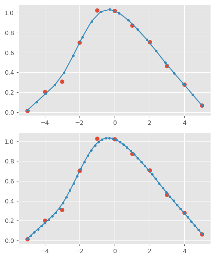
Computing Spline Without Evaluating

If we want to compute spline only without evaluating (smoothing data), we can use the following signatures:

spline = csaps(x, y)
spline = csaps(x, y, smooth)

In this case the smoothing spline will be computed for given data and returned as an instance of ISmoothingSpline based class. After we can use the computed spline to evaluate (smoothing) data for given data sites repeatedly.

The example for univariate data:

x, y = univariate_data(n=11)

spline = csaps(x, y)

xi1 = np.linspace(x[0], x[-1], 20)
xi2 = np.linspace(x[0], x[-1], 50)

yi1 = spline(xi1)
yi2 = spline(xi2)

f, (ax1, ax2) = plt.subplots(2, 1, figsize=(5, 6))
ax1.plot(x, y, 'o', xi1, yi1, '.-')
ax2.plot(x, y, 'o', xi2, yi2, '.-')

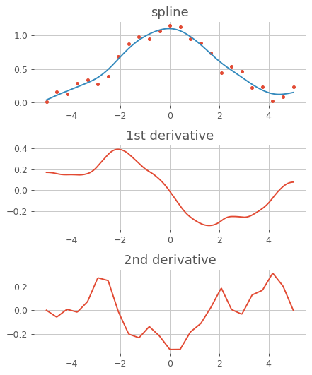
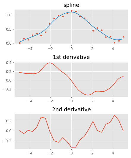
Analysis

We can use spline analysis functionality that is provided by scipy.interpolate.PPoly/scipy.interpolate.NdPPoly classes.

For example, let’s try to use scipy.interpolate.PPoly.derivative() method to compute spline 1st and 2nd derivatives.

from csaps import CubicSmoothingSpline

x, y = univariate_data()
xi = np.linspace(x[0], x[-1], 300)

s = CubicSmoothingSpline(x, y, smooth=0.85).spline
ds1 = s.derivative(nu=1)
ds2 = s.derivative(nu=2)

_, (ax1, ax2, ax3) = plt.subplots(3, 1, figsize=(5, 6))
ax1.plot(x, y, '.', xi, s(xi), '-')
ax2.plot(xi, ds1(xi), '-')
ax3.plot(xi, ds2(xi), '-')

ax1.set_title('spline')
ax2.set_title('1st derivative')
ax3.set_title('2nd derivative')